Algorithms on Graphs: Fastest Route
Key Concepts
We often want to find the shortest path from A to B, where A and B are expressed as nodes, and linked by edges in some graph structure. This simple problem description is non-trivial because of certain properties of the problem and increasingly relaxed assumptions about the problem.
- Are the edges positive, negative, weighted?
- What do we mean by shortest path? Distance travelled? Time taken?
- Are the routes that are blocked? etc.
- We want to do this all as efficiently as possible hence we compare different implementations in the runtime analysis.
Model Preliminaries
- A graph is an abstract representation that models connections between objects. These can be social networks, websites, cities, or even currency exchange paths. We need efficient graph algorithms to compute on graphs, in particular, we are interested in computing shortest paths.
- Formally, a graph $G=(V, E)$ where $V$ are the nodes and $E$ represents the edges.
- We assume adjacency list representation, where each node has a list of its neighboring graphs and the weight or distance of the edge from itself to its neighbors.
Algorithm 1: Breadth-first Search + Shortest Path Tree
Graph properties:
Edges are directed and have equal weight of 1. The shortest path is thus the number of edges traversed.
Intuition:
This algorithm processes nodes with increasing distance away from the starting node. There are two separate steps for this algorithm, 1. Discovery and 2. Processing. New nodes are discovered by processing old nodes. The shortest path can be obtained by backtracking from the target node back to the source.
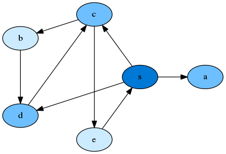
Example where we are provided with the Graph Structure (from an adjacency list). Which can be visualised from a dot file. The start node $s$ explores its neighboring nodes, $c$, $d$, $a$. Nodes which are further away from the source have an increasingly lighter color shade.
Implementation
The algorithm can be implemented with the following:
- Queue: Discovered nodes are processed in First-in-First-Out order
- HashMap1: To store node distances from the source. Nodes only need to be discovered once.
- HashMap2: To store the preceeding node which led to the current node.
import pygraphviz as pgv
import matplotlib.pyplot as plt
from Queue import Queue

class BFS:
  def __init__(self, dotpath):
    self.G = pgv.AGraph(dotpath)
    self.node_d = self._initialise_map(self)
    self.q = Queue()

  def visualise(self):
    self.G.layout(prog="dot")
    self.G.draw('bfs_out.png')
    plt.show()
Initialise the distance hashmap by setting all distances to infinity.
def _initialise_map(self):
  node_d= {}
  for node in self.G.nodes():
    node_d[node]['dist'] = float('inf')
    node_d[node]['prev'] = None
  return node_d
To run the Breadth-first search procedure on any input node, we first enqueue the input node, and set its distance to 0. Next, we process the (source) node and find (target) nodes that are linked to it. If the target nodes have not been explored before, i.e. distance is inf, then we enqueue the target node and (1) update its distance by adding the current node’s distance +1. and (2) keep track of the node that preceeded it.
def run_BFS_from(self, startnode="s"):
  self.q.put(startnode)
  self.node_dist_d[startnode]=0

  while not self.q.empty():
    currentNode = self.q.get()
    for sourceNode, targetNode in self.G.edges():
      if sourceNode == currentNode:
        if self.node_dist_d[targetNode] == float('inf'):
          self.q.put(targetNode)
          self.node_d[targetNode]['dist'] = self.node_d[sourceNode]['dist'] + 1
          self.node_d[targetNode]['prev'] = currentNode
To find the shortest path from node S to node e, we backtrack from e’s previous nodes back to S. Note that we are appending to the list in reverse order, hence we reverse the final result to find the shortest path from S to e.
def get_shortest_path(self, sourceNode="s", targetNode="e"):
  result = []
  while targetNode!=sourceNode:
    result.append(targetNode)
    targetNode = self.node_d[targetNode]['prev']

  return result[::-1]
Runtime analysis
The runtime of breadth-first-search is $O(V+E)$. Of which there is a cute analysis where if $(V)\leq(E)$, then $(V+E)\leq(E+E)=2.E$. Conversely, if $(V)\geq(E)$, then $(V+E)\leq(V+V)=2.V$. Thus $O(V+E)=O(max(V, E))$.
Algorithm 2: Djikstra’s
Graph properties:
Edges are directed and have positive lengths. The shortest path is thus the shortest edge distance traversed (not the number of edges).
Intuition:
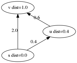
In the course of node exploration, we might discover new node, $u$, that offer a shorter path to a previously discovered node, $v$. When this happens, we should update the distance of the previously discovered node to the new shortest path, and the previously discovered node of $v$ to $u$. The algorithm follows a greedy strategy by repeatedly processing the node with minimum shortest path estimate.
Implementation
To implement the algorithm efficiently, we need mechanisms to:
- Update the order of processing nodes, after their updated distance. The next node to process should have minimum distance value from the starting node. We implement this with a priority queue from the heap data structure and initialise the queue to contain all nodes.
Note: Heapify after adding each node is an $O(n)$ operation. Hence we use the work-around recommended by python docs which does not disrupt the original heap but continuously adds to the heap.
import heapq

class PriorityQueue():
  def __init__(self, nodelist):
    self.entry_finder = {}
    self.REMOVED = '<removed>'
    self.pq = []

    for node in nodelist:
      # Points to the same object such that if entry in entry_finder changes, entry in pq changes.
      entry = [float('inf'), node]
      self.entry_finder[node] = entry
      heapq.heappush(self.pq, entry)

  def update_node(self, node, priority):
    if node in self.entry_finder:
      self.remove_node(node)

    # Again, referencing the same object
    entry = [priority, node]
    self.entry_finder[node] = entry
    heapq.heappush(self.pq, entry)

  def pop(self):
    while self.pq:
      priority, node = heapq.heappop(self.pq)
      if node is not self.REMOVED:
        del self.entry_finder[node]
        return priority, node
raise ValueError('Pop from an empty priority queue')- Update the distance of target nodes $v$, which has outgoing edges from the current node $u$. (i.e relax edge distance from $u$ to $v$)
def relax_edge(self, newNode="u",  oldNode="v"):
  newDist_oldNode = self.node_d[newNode]['dist'] + self.mat[newNode][oldNode]

  if (self.node_d[oldNode]['dist'] > newDist_oldNode):
      self.node_d[oldNode]['dist'] = newDist_oldNode
      self.node_d[oldNode]['prev'] = newNode
      self.PQ.update_node(tNode, newDist_oldNode)
The full implementation follows the spirit of breadth-first search exploration. We pop nodes from the priority queue, find edges that link the source node to target nodes, and check if we can ‘relax edges’ i.e. have any updated distances for the target nodes. If the distance has changed, we update the priority queue. The while loop iterates exactly $|V|$ times, as we add nodes to the priority queue exactly once(although we may update its values). In each iteration, we remove a node from the priority queue until all nodes have been processed.
import networkx as nx

class DjikDemo():
  self.mat = self.load_matrix() # any implementation
  self.G = nx.from_numpy_matrix(self.mat)
  self.PQ = PriorityQueue(self.G.nodes())
  self.node_d = self._initialise_map() # same as in bfs

def run_DJIK_from(self, startnode=0):
  self.PQ.add_node(0, 0)
  self.node_d[startnode]['dist'] = 0
  node = startnode

  while node != self.PQ.REMOVED:
    try:
      priority, node = self.PQ.pop()
    except:
      break
    edges = self.G.edges(node)

    for sNode, tNode in edges:
      self.relax_edge(newNode=tNode, oldNode=sNode)

  print "Distances from start:", [(n, self.node_d[n]['dist']) for n in self.node_d.keys()]
Runtime Analysis
The running time analysis depends on the data structure used to implement the priority queue
- Create the data structure
- Find and extract the next node to process - we need to do this operation $V$ times (once for each node).
- Change the priority of the nodes - we need to do this operation $E$ times (once for each edge).
- Array: $O(V + V^2 + E) = O(V^2)$
- Create takes $O(V)$.
- Find and extract takes $O(V)$, which would be $O(V^2)$ for all operations.
- Change takes $O(1)$ for a single operation, which would be $O(E)$ for all operations.
- Binary Heap (our implementation): $O(V + VlogV + ElogV)$ = $O((V+E)logV)$
- Create takes $O(V)$.
- Find and extract takes $O(logV)$, which would be $O(VlogV)$ for all operations.
- Change takes $O(logV)$ time, which would be $O(ElogV)$ for all operations. In our implementation, the size of the binary heap has a maximum size of $|E|$, which is at most $|V|^2$ if the graph is fully connected. $O(log(V^2))$ = $O(2log(V))$ = $O(logV)$
If $|E|$ is small, then the binary heap implementation is much better than the array. If $|E|$ is close to $|V|^2$, then the array implementation is better because the binary heap runtime becomes $O(V^2logV)$
Algorithm 3: Bellman-Ford
Graph Properties
Graph edges can have directed negative weights. The shortest path thus takes into account negative distances traversed.
Intuition
The Bellman-Ford iterates over the Graph $|V|-1$ times, and relaxes all edges $E$ in the graph at each iteration. Unlike Djikstra’s algorithm which assumes that all edge weights are positive, and can selectively relax edge weights based on the sequence of node explorations (implemented by the priority queue), the Bellman-Ford can not assume the correct sequence of node and edge exploration and hence iterates through everything with brute-force.
Implementation
As a result of the brute-force procedure, the implementation is considerably simpler than Djikstra’s. The algorithm is guaranteed to converge after $|V|-1$ iterations to the right distances if no negative cycles exist. Hence, a convergence check shows whether or not there are negative cycles in the graph.
class BellmanFordDemo():
  def __init__(self):
    self.mat = self._initialise_mat()
    self.G = self._initialise_graph()
    self.node_d = self._initialise_map()

  def run_Bellman_Ford(self, startnode='s'):
    self.node_d[startnode]['dist'] = 0
    for i in range(len(self.G.nodes())):
      for sNode, tNode in self.G.edges():
        # Relax edge
        newDist = self.node_d[sNode]['dist'] + self.mat[sNode][tNode]
        if self.node_d[tNode]['dist'] > newDist:
          self.node_d[tNode]['dist'] = newDist
          self.node_d[tNode]['prev'] = sNode

    self._has_negative_cycle()

  def _has_negative_cycle(self):
    for sNode, tNode in self.G.edges():
      newDist = self.node_d[sNode]['dist'] = self.mat[sNode][tNode]
      if self.node_d[tNode]['dist'] > newDist:
        return False
    return True
Runtime Analysis
The Bellman-Ford runs in $O(V + VE) = O(VE)$ time:
- Initialisation takes $O(V)$.
- The nested for-loop takes $O(VE)$. Iterating over all the edges over the graph takes $O(E)$, and we do this $O(V-1)$ times.
To come..
- A-star
- Bidirectional Djikstra
- Floyd warshall
References
Introduction to Algorithms (CLRS) 24.1-24.3
UCLA and School of Economics(Coursera)