Gibbs Sampling on Dirichlet Multinomial Naive Bayes (Text)

Key Concepts

• Gibbs Sampling is a type of MCMC method, which allows us to obtained in samples from probability distributions, without having to explicitly calculate the values for their marginalizing integrals. The key idea (amongst the other MCMC methods) is to sample each unknown variable in turn, condition on the value of all other variables in the model.

• The Dirichlet Multinomial model is a frequently encountered model in Bayesian Statistics. Here a prior $\theta$ is drawn from a dirichlet distribution, with parameters $\gamma_\theta$, $\theta \sim Dir(\gamma_\theta)$, and the observed values are drawn from a Multinomial distribution with parameters $\theta$ and trials $n$, $V \sim Multinomial(\theta, n)$.

• The Dirichlet distribution is a conjugate distribution to the Multinomial distribution, which has useful properties in the context of Gibbs Sampling.

Model Preliminaries

In Bayesian Inference, the aim is to infer the posterior probability distribution over a set of random variables. However this involves computing integrals which are mostly intractable.

MCMC methods are a way to approximate the value of the integral, by sampling from the joint distribution. (Hence, we never need to calculate explicitly the value of the integral). The idea is to sample from a state space of $Z$ such that the likelihood of sampling $z$ is proportional to $p(z)$. The Markov Chain indicates that the next state, $t+1$, that we visit depends only on the current state, $t$. That is,

\begin{equation} P_{trans}(z^{t+1}|z^{t}) = P_{trans}(z^{t+1}|z^t, z^{t-1}, …, z^1) \end{equation}

MCMC methods try to approximate $P_{trans}(z^{t+1}|z^{t})$ such that the probability of visiting $z$ is proportional to $p(z)$. Values of variables in the model can be approximated from simple statistics. Read more about MCMC [here].

Gibbs Sampling is one type of MCMC method, that applies when $z$ has $k$ dimensions, $z=<z_1, z_2, …, z_k>$ . Each dimension corresponds to a parameter or variable in our model. The algorithm samples from the conditional distribution by updating $z$ one dimension at a time. The probabilistic walk samples each $k$ dimension, condition on the other $k-1$ dimensions. In this process, new values for the variables are used as soon as they are obtained. For each iteration $t$ in $1..T$, sample each $i$ in $1..k$, such that:

\begin{equation} z_i^{t+1} \sim P(z_i^{t+1}|z_1^{t+1}, …, z_{i-1}^{t+1}, z_{i+1}^{t},…, z_k^{t}) \end{equation}

In Probabilistic Graphical models, we seek to infer(through Bayesian inference) probability distributions over latent variables which are parameters in the model. To apply Gibbs Sampling, we need to first obtain the mathematical equations for the conditional updates. The general workflow is as follows:

1. Assume a generative model which allows us to observe the data generated by some latent variables. The model is often constructed with domain knowledge and results in structured joint distributions.
   • Draw the probabilistic graphical model using plate diagram
     
     
2. Factorise the joint distribution of the model to conditional distribution based on the model structure.
   • Express conditional distributions in terms of mathematical equations.
     
     
3. Sample variables by running the Gibbs Sampling algorithm.
   • Obtain equations for conditional update of variables.
     
     
4. Obtain approximate values of the variables via sample statistics.

Implementing Gibbs Sampling on Dirichlet Multinomial Naive Bayes Model

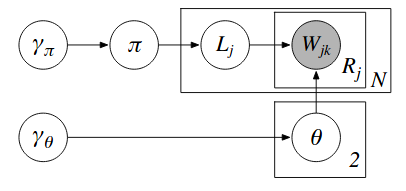
The rest of this document follows the Dirichlet Multinomial Naive Bayes (DMNB) Model from “Gibbs Sampling for the Uninitiated”. The model described in the paper has documents as the item of interest. Each document, $doc_j$, can be represented as a bag of words, $W_j$. The observed features are the words in the document, with the k-th word in the j-th document represented as $W_{jk}$. The goal is to predict a sentiment label $L_j$ for each of the documents, after observing $W_j$. By Bayes Rule,

\begin{equation} L_j = argmax_LP(L|W_j) = argmax_L\frac{P(W_j|L)P(L)}{P(W_j)} \end{equation}

Then, $L_j = argmax_LP(L|W_j, \pi, \gamma_\pi, \theta, \gamma_\theta)$.

1. Assume a generative model of text

Assume a generative model expressed by the following directed graphical model. Sampling from a directed graphical model involves sampling from each node condition on its parents. For top level varibles, this involves sampling from its marginal or providing estimates directly.

• L is a 2-class label, which can be sampled from a Bernoulli distribution with parameter $\pi$ where $P(L_j=1)$. For more than 2 classes, L can be sampled from a multinomial distribution.

\begin{equation} L_j \sim Bernoulli(\pi) \end{equation}

• $\pi$, the parameter of the Bernoulli distribution, is sampled from a conjugate prior probability - the Beta distribution which has hyperparameter $\gamma_\pi = [\alpha, \beta]$. Without any previous information, we use an uninformative prior, $\gamma_\pi = [1, 1]$, which returns a uniform distribution where any value of $\pi$ is equally likely.

\begin{equation} \pi \sim Beta(\gamma_\pi) \end{equation}

• We assumes a Naive model of word generation, where the words generated are independent of each other given L. The probability distribution that the words are sampled from depends on whether $L_j$ is 0 or 1. If $L_j=0$, the probability distribution we sample from is $w_0 \sim Multinomial(\theta_0)$. Generally,

\begin{equation} w_j \sim Multinomial(\theta_{L_j}) \end{equation}

• $\theta_{L_j}$, the parameter of the Multinomial distribution is sampled from a prior probability, the Dirichlet distribution. The Dirichlet distribution is the Beta distribution generalized to more than two possible values. The dirichlet distribution is parameterised by hyperparameter $\gamma_\theta$. The number of dimensions is the number of words in the vocabulary. $\gamma_\theta = [\gamma_{\theta_1}, \gamma_{\theta_2},…,\gamma_{\theta_v}]$

\begin{equation} \theta \sim Dirichlet(\gamma_\theta) \end{equation}

class DMNB(hyp_theta, hyp_pi):
    self.hyp_pi = hyp_pi
    self.hyp_theta = hyp_theta
    self.pi = 0
    self.theta_0 = []
    self.theta_1 = []  

    #def update_label(self, doc, corpus):
    
    #def update_theta(self):

    #def initialise(self):

    #def inference(self, train_corpus, iterations):

2. Factorise the joint distribution

The joint distribution of the model above is $P(C, L, \pi, \theta_0, \theta_1, \gamma_\pi, \gamma_\theta)$ where $C$ represents the entire document collection. $C_0$ and $C_1$ are the set of documents with label 0 and 1 respectively. The independence assumptions based on the graphical model shown in Fig1. give the following conditional distribution:

\begin{equation} P(C_0|L, \theta_0)P(C_1|L, \theta_1)P(\theta_0|\gamma_\theta)P(\theta_1|\gamma_\theta)P(L|\pi)P(\pi|\gamma_\pi) \end{equation}

We need to convert this into it’s mathematical form so that we can perform updates for Gibbs Sampling subsequently. The state space of variables to update is $L, \pi, \theta_0, \theta_1$.

• $P(C_x|L, \theta_x)$ is the probability of observing documents(and its contents) with label $x\in \lbrace0, 1\rbrace$, given label sequence $L$ and $\theta_x$. Since the documents are generated independently of each other, we can multiply the probability of each document, $D_m$, condition on the document’s label$L_m$ and the multinomial-word distribution, $\theta_{L_m}$ specific to the value of the document’s label.
  
  Assuming a Naive Bayes model, the probability of observing the document’s bag-of-words, $w_1,..w_V$, can be obtained from multiplying each word’s probability (document specific), $\theta_{L_m(w_i)}$.

\begin{equation} P(C_x|L, \theta_x) = \prod_{m\/in C_x}{}P(D_m|L, \theta_{L_m}) \end{equation} \begin{equation} = \prod_{m\in C_x}.\prod_{i=1}^{V_m}\theta_{L_m(wi)}^{count(wi)} = \prod_{i=1}^{V}\theta_{L_m(w_i)}^{count(w_i \in C_x)} \end{equation}

• $P(\theta_x|\gamma_\theta)$ is the probability of the multinomial word distribution, drawn from a dirichlet prior with hyperparameter $\gamma_\theta$. By definition,

\begin{equation} P(\theta_{L_m}|\gamma_\theta) = c.\prod_{i=1}^{V}\theta_{L_m(i)}^{\gamma_{\theta_i}-1} \end{equation}

• $P(L|\pi)$ is the probability of obtaining a specific sequence L of N binary labels, given that the probability of choosing label=1 is $\pi$.

\begin{equation} P(L|\pi) = \pi^{C_1}(1-\pi)^{C_0} \end{equation}

• $P(\pi|\gamma_\pi)$ is the probability of drawing $L$ given the prior Beta distribution with hyperparameters $\gamma_\pi=[\alpha,\beta]$. By definition of the Beta distribution, where c is a normalization constant:

The factorised joint distribution is thus,

\begin{equation} c.\prod_{i=1}^{V}\theta_{1(w_i)}^{count(w_i\in C_1)+\gamma_{\theta_i}-1}\prod_{i=1}^{V}\theta_{0(w_i)}^{count(w_i\in C_0)+\gamma_{\theta_i}-1}.\pi^{C_1+\alpha-1}(1-\pi)^{C_0+\beta-1} \end{equation}

2.1 Integrating out $\pi$

We would like to simplify the problem by reducing the number of variables to sample. To do this, we can integrate out $\pi$ from the joint distribution, which has the effect of taking all possible values of $\pi$ into account without representing it explicitly at every iteration. That is,

We can get rid of the integral by substituting the true distributions for $P(\pi)$ from eqn(12) and $P(\pi|\gamma_\pi)$ from eqn(13).

\(\begin{align} \int_{\pi}P(\pi).P(\gamma_\pi)d\pi = \int_{\pi}\pi^{C_1}(1-\pi)^{C_0}.\frac{\Gamma(\alpha+\beta)}{\Gamma(\alpha)\Gamma(\beta)}\pi^{\alpha-1}(1-\pi)^{\beta-1}d\pi \nonumber \\\ = \frac{\Gamma(\alpha+\beta)}{\Gamma(\alpha)\Gamma(\beta)}.\int_{\pi}\pi^{C_1+\alpha-1}(1-\pi)^{C_0+\beta-1}d\pi \end{align}\) Observe that the second part of this eqn is the beta distribution.

\begin{equation} = \frac{\Gamma(\alpha+\beta)}{\Gamma(\alpha)\Gamma(\beta)}.\int_{\pi}Beta(C_1+\alpha,C_0+\beta)d\pi \end{equation}

The value of the integral of the Beta distribution is given by the normalizing constant. Hence,

\begin{equation} = \frac{\Gamma(\alpha+\beta)}{\Gamma(\alpha)\Gamma(\beta)}.\frac{\Gamma(C_1+\alpha)\Gamma(C_0+\beta)}{\Gamma(C_0+C_1+\alpha+\beta)} \end{equation}

Substituting eqn (18) back into the joint distribution gives us,

\begin{equation} c.\prod_{i=1}^{V}\theta_{1(w_i)}^{count(w_i\in C_1)+\gamma_{\theta_i}-1}\theta_{0(w_i)}^{count(w_i\in C_0)+\gamma_{\theta_i}-1}.\frac{\Gamma(\alpha+\beta)}{\Gamma(\alpha)\Gamma(\beta)}.\frac{\Gamma(C_1+\alpha)\Gamma(C_0+\beta)}{\Gamma(C_0+C_1+\alpha+\beta)} \end{equation}

3. Obtain equations for conditional update of variables

In this model (see plate diagram) - the document words, $W_{jk}$ are observed, and $\gamma_\pi, \gamma_\theta$ are hyperparameters of the model. $\pi, L, \theta_0, \theta_1$ are parameters of the model that need to be sampled. Having integrated out $\pi$, we are left with:

• $L$ is the binary label variable which must be sampled for each document
• $\theta_0, \theta_1$ is the probability of drawing a word from a multinomial distribution if the label of the document is 0 or 1 respectively. It is a vector with length $|V|$, where $V$ is the vocabulary.

To assign the value of $L_2^{(t+1)}$, we need to sample from the conditional distribution of \begin{equation} P(L_2|L_1^{(t+1)},L_3^{(t)},..,L_N^{(t)}, C, \theta_0^{(t)}, \theta_1^{(t)}; \gamma_\theta, \gamma_\pi) \end{equation}

To assign the value of $\theta_0^{(t+1)}$, we need to sample from the conditional distribution of \begin{equation} P(\theta_0|L_1^{(t+1)}, .., L_N^{(t+1)}, C, \theta_1^{(t)}, \gamma_\theta, \gamma_\pi) \end{equation}

To help us with all the counts, we create document and corpus classes that can be easily re-used for texxt models related to probabilistic MCMC updates.

3.1 Conditional update of $L_j$

For each document in the corpus, we need to draw the update from a single Bernoulli trial. In order to do that, we need to get the relative probabilities of $P(L_j=x |..)$ for $x \in \lbrace 0,1 \rbrace$, as the parameter for the Binomial distribution.

\begin{equation} val0 = P(L_j=0|L_{(-j)}, C_{(-j)}, \theta_0, \theta_1, \gamma_\pi, \gamma_\theta) = \frac{C_0+\gamma_{\pi_0}-1}{C_0 + C_1 + \gamma_{\pi_1}+ \gamma_{\pi_0} -1}.\prod_{i=1}^{V}\theta_{0}^{W_{ji}} \end{equation}

\begin{equation} val1 = P(L_j=1|L_{(-j)}, C_{(-j)}, \theta_0, \theta_1, \gamma_\pi, \gamma_\theta) = \frac{C_1+\gamma_{\pi_1}-1}{C_0 + C_1 + \gamma_{\pi_1} + \gamma_{\pi_0} -1}.\prod_{i=1}^{V}\theta_{1}^{W_{ji}} \end{equation}

\begin{equation} L_j \sim Binomial(\frac{val0}{val0+val1}) \end{equation}

from numpy.random import binom

class DMNB(hyp_theta, hyp_pi):
... 

  def update_label(self, corpus, doc):

    pL0 = np.log(corpus.doc_label_m.sum(axis=0)[0] + self.hyp_pi[0] - 1)
    pL1 = np.log(corpus.doc_label_m.sum(axis=0)[1] + self.hyp_pi[1] - 1)

    for word in doc.word_label:
      pL0 += np.log(self.theta_0[word_ix])
      pL1 += np.log(self.theta_1[word_ix])

    pL0 = np.exp(pL0)
    pL1 = np.exp(pL1)

    L = binom(pL1/(pL0+pL1))

    return  L

3.2 Conditional update of $\theta_0$ and $\theta_1$

For $\theta_0$ and $\theta_1$, we also need to sample new distributions condition on all other variables. However since we used conjugate priors, the posterior, like the prior, is a dirichlet distribution. The use of conjugate priors simplifies the update as we can draw a new $\theta_x$, where $x \in \lbrace 0, 1\rbrace$ by adding pseudocounts to the hyperparameter of the dirichlet prior:

\begin{equation} \theta_x \sim Dirichlet([(count(w_i\in C_x) + \gamma_{\theta_x(i)}), … , (count(w_v\in C_x)+\gamma_{\theta_x(v)})]) \end{equation}

from numpy.random import dirichlet

class DMNB(hyp_theta, hyp_pi):
... 
  def update_theta(self, corpus):
    
    new_hyp_theta_0 = []
    new_hyp_theta_1 = []

    for word in self.vocab_ix:
      w = self.vocab_ix[w]
      new_hyp_theta_0.append(corpus.word_label_m[w][0] + self.hyp_theta)
      new_hyp_theta_1.append(corpus.word_label_m[w][1] + self.hyp_theta)

    self.theta_0 = dirichlet(new_hyp_theta_0)
    self.theta_1 = dirichlet(new_hyp_theta_1)

4. Sample variables by running the Gibbs Sampling algorithm

4.1 Initialization

The state space of which we need to sample includes

• $\pi$, sampled once from a beta distribution and re-used for each draw of $L$.
• $L$, binary label variables, one for each document,
• $\theta_0, \theta_1$, sampled once from a dirichlet distribution

from scipy.stats import binom
from numpy.random import beta, dirichlet

class DMNB(hyp_theta, hyp_pi):
...
  def initialise(self, corpus):

    pi = beta(self.hyp_pi)
    self.labels = binom(1, pi).rvs(len(corpus.docs))
    self.theta_0 = dirichlet(self.hyp_theta)
    self.theta_1 = dirichlet(self.hyp_theta)

4.2 Algorithm

There are two for-loops for the variable update.

The inner loop predicts a new label for each document $j=1..N$, we

• remove counts associated with document j,
• assign a new label to it from Section 3.2
• add counts associated with the new label.

For the outer loop, iterations $t=1…T$,

• we draw a new distribution for $\theta_0$ and $\theta_1$.

class DMNB(hyp_theta, hyp_pi):
...

  def gibbs_inference(self, train_corpus, iterations):
    for t in range(iterations):
      for doc in train_corpus.docs:
        corpus.doc_label_m[doc][0]=0
        corpus.doc_label_m[doc][1]=0
        self.update_label(train_corpus, doc)
        corpus.doc_label_m[doc][L]=1
        
      self.update_theta()

Note that: once a new label is assigned, it changes the counts that affect the labeling of the subsequent documents.

Calculating Sample Statistics

According to MCMC theory, an estimate of the desired variable can be obtained by averaging across all samples obtained so far. Optionally, there is also

• Running independent Gibbs sequences and averaging the final value of each sequence.
• Discarding burn-in samples
• Autocorrelation and lag
  • Variations on Gibbs sampling aim to reduce autocorrelation
• Sampling the last value - Under reasonably general conditions, the distribution of the samples drawn converges to the through distribution. Thus for a large enough number of iterations, the final observation is effectively a sample point from the true distribution.

References

Resnik, P., & Hardisty, E. (2010). Gibbs sampling for the uninitiated