Likelihood weighted Sequential Importance Sampling

Sequential Monte Carlo (SMC) methods are a set of Monte Carlo algorithms used to solve filtering problems arising in signal processing and Bayesian statistical inference.

The main idea of Monte Carlo methods is that we can get a (monte carlo) approximation of the distribution $p$ from samples drawn from $p$. Imagine that we are provided with samples from a probability distribution, but we don’t know what the probability distribution is. We can plot the histogram (density) of the samples, which is equivalent to:

Assuming a discrete distribution, the probability of a discrete outcome $x$, is the proportion of times that outcome has occurred (denoted by the delta function $\delta_x^{(i)}(x)$). Below we draw 10000 samples from a mystery distribution, from which we can calculate some sample statistics.

import numpy as np
import matplotlib.pyplot as plt
from scipy.stats import rdist, norm, logistic, maxwell
mystery = norm # imagine you can't see this

samples = mystery.rvs(size=10000, scale=1)
plt.hist(samples, density=True)

In importance Sampling, we don’t know how to draw from $p$. However, the trick is to approximate a target distribution $p$ that we cannot draw samples from, with samples $x$ drawn from a “proposal distribution” $q$. The assumption is that we can evaluate both $p(x)$ and $q(x)$, and we can draw $x\sim q(x)$ easily (in closed-form). Importance sampling relies on the fundamental identity (Robert and Casella, 2004).

For each sample drawn, we need to account for the difference in $p$ and $q$, by reweighting that sample by $p(x)/q(x)$. Strictly speaking, Importance Sampling is not a way to sample, but is a way to REWEIGHT samples from a proposal distribution (that we can sample from).

To plot the histogram distribution, we binning all the sample ($x$) values, and reweighting the “frequency” of that sample by $\hat{w} = \frac{p(x)}{q(x)}$. The actual weight still requires normalisation across all $i$ samples: $w_i = \frac{\hat{w_i}}{\sum_{j=1}^N \hat{w_j}}$

def importance_sampling(sample_size, bin_size=0.1, p_dist="", q_dist=""):
  # first draw samples from q distribution that is easy to draw from
  samples = q_dist.rvs(size=sample_size)
  p = lambda x: p_dist.pdf(x, c=1.6)
  q = lambda x: q_dist.pdf(x)

  bin_positions = np.arange(min(samples)-bin_size, max(samples)+bin_size, bin_size)
  p_bin_heights = np.zeros(len(bin_positions))
  q_bin_heights = np.zeros(len(bin_positions))

  # normalise weights
  weights = []
  for i, sample in enumerate(samples):
    weights.append(p(sample)/q(sample))
  weights = weights/np.sum(weights)
  
  # binning values
  for i, sample in enumerate(samples):
    bin = np.where(sample<bin_positions)[0][0] 
    p_bin_heights[bin] += weights[i]  
    q_bin_heights[bin] += 1/len(samples)

  #print(q_bin_heights)
  return p_bin_heights, q_bin_heights, bin_positions, samples

Below, blue is the histogram of points drawn from the $q$ distribution (without reweighting), and orange is the resulting histogram after importance reweighting. The more samples, the better the estimate, so clearly, if we have drawn more samples that are in the target distribution, then we would get better representation under this distribution. Similarly, using a proposal distribution that is closer to the target distribution would give us a better approximation.

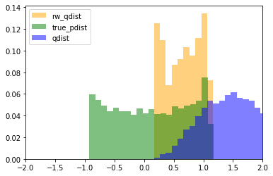
Importantly, the support of the proposal distribution that we sample from must cover the target distribution. i.e, $q(x)>0$ whenever $p(x)>0$. If we had used a different distribution that did not cover the support of the target, then we cannot approximate the target at all under those samples. In the example below, we our samples are drawn only from the $[0,1]$, and the resulting approximation of the target distribution is(orange) “empty” at values below 0. The true target distribution is given by green.

Deriving likelihood weighted Sequential Importance Sampling for HMMs

In Sequential Importance Sampling (aka Particle Filtering without resampling), our $N$ samples through time are represented as particles denoted as $v_i$, which will need to be reweighted according to the proposal distribution.

Many courses (the famous Berkeley CS188 Intro to AI course and everyone else who copies their material) directly teach this together with HMMs, and describe particles as a series of states sampled from the transition distribution, and give the corresponding incremental weight updates of the form:

$w_t(v_i) = p_{\text{emission}}(y_t |x_t) \times w_{t-1}(v_i)$

calling this “likelihood weighted sampling”. The rest of this post shows how to derive likelihood weighted sampling for HMMs, from first principles, so that we will hopefully know how to do this for other models.

Note: $x_t$ denotes hidden states at time $t$, while $y_t$ denotes observed states, following notation from Doucet and Johansen (2009).

In state space models, we only know the target distribution up to a normalising constant. The target distribution: $p(x_{1:T}|y_{1:T})$ is expressed as:

\begin{align} p(x_{1:T} | y_{1:T}) = \frac{p(x_{1:T}, y_{1:T})}{p(y_{1:T})}= \frac{\gamma_T(x_{1:T})}{Z} \end{align}

The weight for the entire particle sequence is given by reweighting by the term $\frac{p(x)}{q(x)}$ as in the first equation of the blog post, where $p(x)=\gamma(x_{1:T})$, and $q(x)=q(x_{1:T}|y_{1:T})$. For an optimal or exact sampler we would transition to state $x_t$ by sampling from the distribution $q^{opt}(x_t | x_{1:t-1}, y_{1:t})$.

The general form of the weight increment before normalisation at $t=3$ is:

Generalising from eq(2), the general form of the weight increment ($\rho_t$) is given by:

Applying conditional independence assumptions of HMMs for the proposal distribution

For regular HMM the joint distribution, which is the numerator on the RHS of the incremental weight is:

\begin{equation} \label{eq:hmm} \gamma_n (x_{1:n})=p(x_{1:n}, y_{1:n}) = p(x_1) \prod_{t=1}^n f(x_t | x_{t-1}) \prod_{t=1}^n g(y_t | x_t) \end{equation}

The HMM model makes conditional independence assumptions for each state at time $t$ to be independent of states $<{t-1}$. Instead of our exact sampler $q^{opt}$, we use a simpler proposal distribution, $q^{\text{hmm}}=f(x_t|x_{t-1})$, which are the transition probabilities of the HMM. With these simplifying assumptions, the incremental update of $\rho_t$ becomes:

which gives us the textbook likelihood weighted importance sampling.

In general for Sequential Importance Sampling, once we have the proposal distribution as determined by the model design and worked out the corresponding reweighting equation(we showed how to do this for HMMs), implementing it is very straightforward; here’s the py pseudocode

for t in range(timesteps):
  for n in range(num_particles):
    particles[n].sample_new_state_from_proposal_distribution()
    particles[n].reweight_sample()

  for n in range(num_particles):
    particles[n].normalise_weights()

  # Optionally Resample 
# Gather Statistics from the Particles

As a final note, resampling of particles is what makes this method “Particle Filtering”. Berkeley CS188 covers this pretty well with nice graphics.

References

Berkerley CS188: HMMs and Particle Filtering

Casella, G., Robert, C. P., & Wells, M. T. (2004). Mixture models, latent variables and partitioned importance sampling. Statistical Methodology, 1(1-2), 1-18.

Doucet, A., & Johansen, A. M. (2009). A tutorial on particle filtering and smoothing: Fifteen years later. Handbook of nonlinear filtering, 12(656-704), 3.