Lagrange Multipliers and Constrained Optimization
Intuition
-
The method of lagrange multipliers is a strategy for finding the local minima and maxima of a differentiable function, $f(x_1, … , x_n):\mathbb{R}^n \rightarrow \mathbb{R}$ subject to equality constraints on its independent variables.
-
In constrained optimization, we have additional restrictions on the values which the independent variables can take on. The constraints can be equality, inequality or boundary constraints. The lagrange multiplier technique can be applied to equality and inequality constraints, of which we will focus on equality constraints.
-
Equality constraints restrict the feasible region to points lying on some surface inside $\mathbb{R}^n$. The constraint can be expressed by the function $g(x_1, …, x_n)$, and points which satisfy our constraint belong to the feasible region. These are the points $x$ where $g(x)=0$.
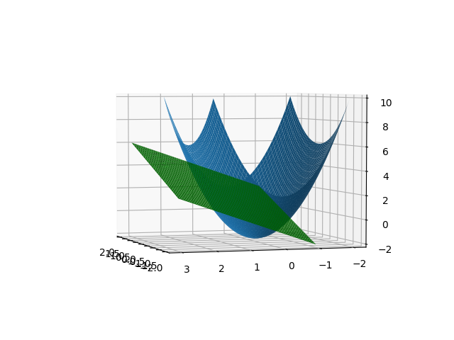
- The point at which the function and constraint are tangent to each other, i.e. touch but do not cross is the solution to the maximum or minimum of the optimization problem. The intuition is that $f$ cannot be increasing or decreasing in the direction of any neighboring point in the feasible region of $g$. If $f$ and $g$ were non-tangent and crossing, then we could always increase or decrease $f$, while satisfying the constraint $g$.
Mathematical Formulation
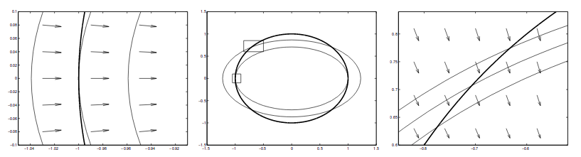
- When two functions/curves are tangent at a point $p$, their normal vectors, or gradients, are parallel at that point $p$.
 |
|---|
| Image from Klein, Langrage multipliers without permanent scarring |
- Because the gradients are pointing in the same direction but not necessarily equal, they can be expressed by the following equation where $\lambda$ is known as the “lagrangian multiplier”.
\begin{equation} \nabla f(p) = \lambda \nabla g(p) \end{equation}
- Together with the original constraint, $g=0$, this gives us sufficient equations to solve for $p$. We can express this compactly with an equation known as the ‘Lagrangian’:
\begin{equation} L(p, \lambda) = f(p) - \lambda g(p) \end{equation}
- Solving for eq(1), is equivalent to solving:
\begin{equation} \nabla L(p, \lambda) = \nabla f(p) - \lambda \nabla g(p)= 0. \end{equation}
- Working out an example where $f=2-x_1^2+2x_2^2$, and $g=x_1^2+x_2^2-1$, amounts to solving $n+1$ equations with $n+1$ unknowns. (There are $n$ independent variables and one lagrangian multiplier, $\lambda$.)
- The solution for the constrained problem is obtained when solving for the points where the partial derivatives of $L$ are zero. Solving for the stationary point of the Lagrangian indicates that the gradient $\nabla f(p)$ does not have to be 0 at the solution, but it should be contained in the subspace spanned by $\nabla g(p)$.
Generalising to multiple constraints
-
Generalizing this to multiple constraints, $g_i(x)=0$, where $g_i$ is the $i$-th constraint, the solutions $p$ must satisfy each $g_i(p)=0$.
-
Geometrically, this means that $\nabla f(p)$ must be entirely contained in the subspace spanned by the $\nabla g_i(p)$ normals. This translates to $\nabla f(p)$ being a linear combination of the gradients of each constraint $g_i(x)$, with weights $\lambda_i$.
\begin{equation} \nabla f(x) = \sum_i\lambda_i\nabla g_i(x) \end{equation}
-
A crucial difference to note from the single constraint case, is that the solution is no longer found at the point where two functions are tangent to each other. The solution is now found when $\nabla f$ is parallel to a combination of the normal vectors of the constraints, $\sum_i \lambda_i\nabla g_i$
-
The Lagrangian for the multiple constraint case then becomes a function of $n+m$ variables ($x\in \mathbb{R}^n$ and $m$ of $\lambda_i \in \lambda$). Differentiating $L$ gives $n+m$ equations, which are solved by setting the partial derivative to zero.
\begin{equation} L(x, \lambda) = f(x) - \sum_i\lambda_ig_i(x) \end{equation}
- Note that differentiating $L(x, \lambda)$ with respect to $\lambda_i$, and solving the equation wrt $0$ gives the $i$-th constraint, $g_i(x)=0$.
Meaning of the Lagrangian multiplier, $\lambda$
-
From eq(1), we can see that $\lambda$ is the amount $L$ would change, for every one unit of $x$ in constraint $g$. The multiplier is also the value of the partial derivative of $L$ wrt to $g_i$, thus it is the rate at which $L$ would increase if the constraint value is raised (aka if the constraint is relaxed).
-
If $\lambda$ is positive, then the objective function will change in the same direction as the constraint value. If $\lambda$ is negative, then the objective function will change in the opposit direction as the constraint value.
-
The interpretation of the lagrange multiplier in nonlinear programming problems is analogous to the dual variables in a linear programming problem.
Lagrangian duality
- The Lagrangian dual function is Concave because the function is affine in the lagrange multipliers.
Lagrange Multipliers and Machine Learning
-
In Machine Learning, we may need to perform constrained optimization that finds the best parameters of the model, subject to some constraint. An example is the SVM optimization problem.
-
To solve the optimization, we apply Lagrange multiplier methods to modify the objective function, through the addition of terms that describe the constraints. The new function to optimize thus becomes the original function plus the constraints, with each constraint weighted by a Lagrange multiplier $\lambda$ which indicates how much to emphasize the constraint.
- Regularized least squares
- Maximum margin classifiers
- Model Comparison
- Linear Discrimant Analysis
Lagrange Multipliers and Information Theory
The lagrangian is applied to enforce a normalization constraint on the probabilities.
Advantages and Disadvantages of the method
The Lagrange multiplier method can be used to solve non-linear programming problems with more complex constraint equations and inequality constraints. However the method must be altered to compensate for inequality constraints and is practical for solving only small problems.