Taylor Series approximation, newton's method and optimization
Taylor Series approximation and non-differentiability
-
Taylor series approximates a complicated function using a series of simpler polynomial functions that are often easier to evaluate. The key idea is to use a series of increasing powers to express complicated yet well-behaved (infinitely differentiable and continuous) functions.
-
For univariate functions, the first-order polynomial approximates $f$ at point $P$ as a straight line tangent to $f$ at point $P$. The second-order polynomial approximates $f$ as a quadratic equation whose line passes through point $P$. Increasing powers of polynomial result in better approximations to complicated functions.
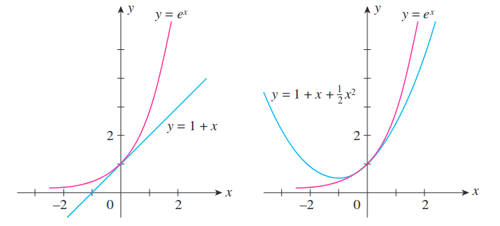 Image taken from Applied Calculus for the Managerial, Life and Social Sciences 8th ed
- At any arbitary point $p$, we use our knowledge of what $f(p), f’(p), f’'(p)$ etc looks like in order to approximate $f(x)$. The Taylor series approximation can be written as:
- This can be equivalently expressed as $f(x_p+\Delta x)$, where $x_p$ is the point where the derivatives are evaluated, and $(x_p+\Delta x)$ is the new point which we wish to approximate. Then,
\begin{equation} f(x_p+\Delta x) = \sum_{n=0}^{\infty} \frac{1}{n!}f^n(x_p)(\Delta x)^n \end{equation}
-
Expected error of Taylor Series [Under construction]
-
For multivariate functions, the Taylor series can be expressed in terms of the Jacobian and Hessian, which reflect the interaction of the first-order derivatives of $J$ and second-order derivatives of $H$ with the $\Delta X = [\Delta x_1, \Delta x_2, … \Delta x_n]$
\begin{equation} f(X_p+\Delta X) = f(X_p) + J_f\Delta X + \frac{1}{2}\Delta X.H_f\Delta X + … \end{equation}
- Tangent Hyperplane: For multivariate functions, the truncated first-order taylor series approximation of a multivariate function $f$ at point $P$ is a hyperplane tangent to $f$ at point P. That is, for $x, \bar{x} \in \mathbb{R}^n$, the tangent hyperplane is given by:
\begin{equation} f(\bar{x}) + \nabla f(\bar{x})^T(x-\bar{x}) \end{equation}
- Taylor series are used to minimise non-differentiable functions. We find a posiiton where we can differentiate the function, and use it to find an approximation of where the function will be at the minimum. This often involves truncating Taylor series polynomials and can be thought of as a ‘linearisation’ (first-order) or quadratic approximation (second-order) of a function.
Newton’s method, root finding, and optimization
- Newton’s method is an iterative method for approximating solutions (finding roots) to equations. If $f$ is a positive definite quadratic function, Newton’s method can find the minimum of the function directly but this almost never happens in practice.
- Instead, Newton’s method can be applied when the function $f$ is not truly quadratic but can be locally approximated as a positive definite quadratic. Given an initial guess $x_0$, Newton’s method makes use of the derivative at $x_0$, $f’(x_0)$ to approximate a better guess $x_1$. Through iteratively applying better guesses, the method constructs a sequence of steps that converges towards some $x$ satisfying $f’(x)=0$.
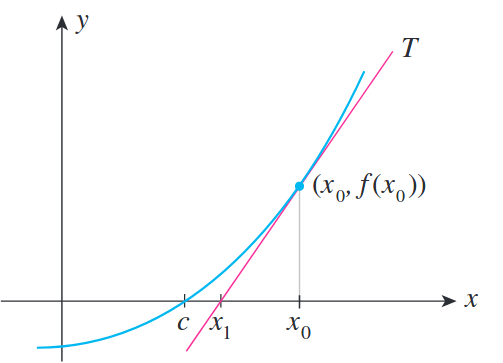 Image taken from Applied Calculus for the Managerial, Life and Social Sciences 8th ed
-
Recall that the Taylor Series approximates $f(x)$ by polynomials of increasing powers, $f(x_p+\Delta x) = f(x_p)+f’(x_p)\Delta x + \frac{1}{2}f’'(x_p)\Delta x^2 + … $
-
We want to find $\Delta x$ such that $(x_p + \Delta x)$ is the solution to minimizing the equation, i.e. $(x_p+\Delta x)$ is the stationary point. To get an estimate of $x$ when $f’(x)=0$, we can truncate the second-order Taylor polynomial, and solve by setting the derivative to $0$.
- Let our initial estimate and the point where we evaluate the derivatives of $f$ be $x_0$. Then the new estimate becomes
- $x_1$ becomes our new estimate, and we can find the next update by $x_2 = x_1 - \frac{f’(x_1)}{f’‘(x_1)}$. This eventually converges to a point $x_n$ which satisfies $f’(x_n)=0$.
Optimization: Newton’s method, Taylor series, and Hessian Matrix
-
In optimization problems, we wish to solve for derivative $f’(x)=0$ to find stationary/critical points. Newton’s method is applied to the derivative of a twice-differentiable function. The new estimate $x_1$ is now based on minimising a quadratic function approximated around $x_0$, instead of a linear function.
-
For the single variable case, we saw that $x_1 = x_0 - \frac{f’(x_0)}{f’'(x_0)}$. We can generalize this to the multivariate case by replacing the derivative $f’(x_0)$ with the gradient, $\nabla f(x)$, and the reciprocal of the second derivative $\frac{1}{f''(x_0)}$ with the inverse of the Hessian matrix, $Hf(x_0)^{-1}$.
\begin{equation} x_1 = x_0 - [Hf(x_0)]^{-1} \nabla f(x_0) \end{equation}
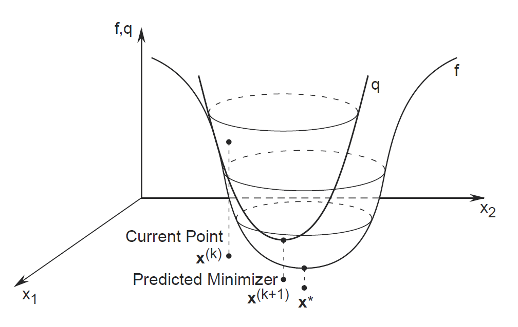 Image taken from: http://netlab.unist.ac.kr/wp-content/uploads/sites/183/2014/03/newton_method.png
- Second-order methods often converge much more quickly but it can be very expensive to calculate and store the inverse of the Hessian matrix. In general, most people prefer quasi-newton methods to approximate the Hessian. These are first order methods which need only the value of the error function and its gradient with respect to the parameters. This can even be better than the true Hessian, because we can constrain the approximation to always be positive definite.