NEURIPS 2020
First timer to the community, thought that main papers were probably too advanced for me to follow. So I spent most of my time checking out (hiding in) the tutorials.
Tutorials
PERSPECTIVES ON NEUROSYMBOLIC ARTIFICIAL INTELLIGENCE RESEARCH
This was actually a workshop but I only listened to the tutorial bits of it.
Neural symbolic approaches aim to enhance module reusability and logical reasoning. Existing approaches tend to maintain two representations, both neural and symbolic logic simultaneously. There are also neural models which provide approximations to logic with no clear guarantees. Logic is language like, some parts of the model are reusable and compositional, but most of the existing implementations don’t have this.
But can neural = symbolic? Put in another way, can we solve a logical system with just neural networks?
When the output of the NN is strictly 1 or 0, there is a direct connection with Boolean logic gates [1], but what about differentiable neurons?
It turns out that there are multiple rigorous real-value logics which have been previously defined, and they vary for the in between values of 0 and 1. For e.g for Godel logic, the OR gate corresponds to $max(a, b)$, and AND gate corresponds to $min(a,b)$. Whereas for Lukasiewicz logic, OR corresponds to $min(1, a+b)$ and AND corresponds to $max(0, a+b-1)$. Interestingly, Lukasiewicz logic corresponds to a RELU. The next ingredient we need is to make weighted versions to weight the importance of different subformulas. For example in Lukasiewicz logic OR gate, we could have $min(1, w_a a + w_b b)$.
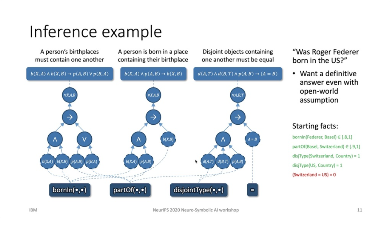
The goal is to answer questions of the form “Does a theory $\Gamma = \{\gamma_1, \cdots, \gamma_n\}$ entail a sentence $\phi$, where $\phi = \{\sigma_1, \cdots, \sigma_k\}$ are lists of formula or primitives associated with a set of candidate truth values $S \subseteq [0, 1]^k$. This decision procedure is known to be NP-hard.
Logical Neural Networks [2] are a neural net style solver, where each neuron is a connective and an atom, and the number of dimensions for each neuron is the number of free variables in the formula. Each is a truth value $\in [0,1]$. The forward pass carries out forward inference, while the backward pass is analogous to the inverse (modus ponens in classical logic). There is a guaranteed convergence because of monotonic tightening in truth value bounds with the forward and backward pass.
[1] McCulloch, W. S., & Pitts, W. (1943). A logical calculus of the ideas immanent in nervous activity. The bulletin of mathematical biophysics, 5(4), 115-133.
[2] Riegel, R., Gray, A., Luus, F., Khan, N., Makondo, N., Akhalwaya, I. Y., … & Ikbal, S.
(2020). Logical Neural Networks. arXiv preprint arXiv:2006.13155.
EQUIVARIANT NETWORKS
Equivariance is something which we explicitly design into our network architectures which makes learning more efficient and generalisable. Equivariance means the symmetry at each layer of the network is preserved. A symmetry is a transformation that leaves some aspect of the object invariant, such as a translation. If the input is translated, then the output feature map is also translated.
This is desirable because later layers can exploit the symmetry (parameter sharing). The convolution layer is CNN is one famous example.
We can define the symmetry transformation of the label function $g$ is a symmetry of $L$, if it satisfies $L \circ g = L$, where $L: X \rightarrow Y$, and $ g: X \rightarrow X’$. This means after applying the transformation $g$, $L$ still gets us the same result.
If we know the transformations that are applied to our data, then we know the set of all data points that you can get by applying this transformation, known as the “orbit”. $O_x = \{g(x) | x \in X, g \in G\}$. $G$ is a “transformation group”, which is a set of transformations that contain the identity transformation, its composition is associative, and the inverse exists. An example is rotations.
Now, if this orbit $O_x$ is a symmetry of our learning problem $L$, then all the points in each of the orbits should be mapped to the same label. We don’t need to learn a separate function for each data point, we just need to learn the mapping for each orbit!
What about just mapping all the points in the orbit to a single point in the feature space? (This is known as Invariance) We can, but this might be premature result in a loss of information for relative positions (the explanation given was kind of hand wavy but I accept it intuitively).
A group representation is a mapping $\rho$, from a group to a set of linear operators or matrices, which can then act on the feature space. The mapping needs to be a homormophism, satisfying this equation $\rho(g2g1) = \rho(g2)\rho(g1)$, where $g2g1$ is the product of two group elements. E.g, if we wanted to swap elements 1 and 2, $P_{12}$ of a vector $v$, then $\rho(P_{12})$ would return us a matrix, which when applied to the vector $v$, does exactly that.
Formally, a network is equivariant, if $f_i \circ \rho_{i-1}(g) = \rho_i(g)\circ f_i$ in the diagram above. In english, a network is equivariant if we first apply a transformation $\rho_{i-1}(g)$ to $X$, followed by a ff $f_i$, and the resulting representation is equivalent to first doing the ff $f_i$, and applying the transformation (which would look different at a different layer), $\rho_i(g)$.
Did not understand the following well enough to write about it
- Steerable CNNs/Harmonic Network
- Gauge symmetry and Gauge CNNs
- Equivalence and Reducibility
- Designing equivariant neurons and Clebsch-Gordon nonlinearity
- Fourier Theory and Generalized convolutions
ABSTRACTION AND REASONING
We know the concept of generalisation intuitively in ML, but can we quantify this? This tutorial introduced the concept of “conversion ratio” which is the efficiency at which we utilise past examples to novel unknown situations, i.e., how well we can generalise. A more intelligent system is one that has a higher conversion ratio.
Abstraction is the key to generalisation, and intelligence is high sensitivity to similarities and isomophisms of the world, and the ability to recast old patterns into a new context. The complexity of our environments is a result of repetition, composition, transformation and instantiation of a small number of “kernels of structure”. Abstraction is being able to mine past experiences for these reusable kernels of structure.
There are two types of abstractions, perceptual representations (which nns are great at doing) and program centric abstractions, like learning how to sort a list (which requires discrete programs). In Deep learning, we are learning a smooth morphing between two geometric spaces. (input to output), in contrast the program abstraction is grounded not in geometry, but in topology. Topology comes about because program synthesis involves a combinatorial search over graphs of operators.
How do we solve tasks which involve program centric abstractions / discrete reasoning? Program synthesis is a combinatorial search over graphs of operators, taken from a domain specific language, with the feedback signal being correctness check. The key challenge is combinatorial explosion and we need to somehow restrict the decision space via heuristics. A nice heuristic to reduce the search space is to identify subgraph isomorphisms in solution programs, abstract this into reusable functions, and add this to the space of repository functions.
Some additional fun things that I noted are:
- The better we can define what we optimize for (more task specific), the less generalization we will achieve because the model will take ‘shortcuts’ to learning without displaying any intelligence.
- Deep learning enables efficiency in learning/optimization in the continuous space through modularity and hierarchy (layers), and reusability (convolution, RNN), together with feedback signals (residual connections).
- The ability to do value abstractions relates to the manifold hypothesis. The manifold hypothesis is that real world high dimensional data, lie in low dimensional manifolds that have been embedded in high dimensional space. If we have found the mapping to this low dimensional manifold, then we have found the correct abstraction that interpolates between two data points. In order for deep learning to work, the manifold hypothesis should apply otherwise we will just be memorising.
- We should test our programs on many instantiations of the same concept and try to do more complex versions of the same task.
Skipped: Deep Learning for Mathematical Reasoning
Practical Uncertainty Estimation and Out of Distribution Robustness in Deep Learning
We care about Out-of-distribution robustness, this is the case when the test and training distribution are different $p_{text}(y,x) \neq p_{train}(y,x)$. While it is unreasonable to be robust to all o.o.d settings, there are some common cases which we would like to be robust to.
- Covariate shift: The distribution of features $p(x)$ changes, but $p(y|x)$ does not change.
- Open-set recognition: new classes may appear at test time.
- Label shift: the distribution of labels $p(y)$ changes, but $p(x|y)$ is fixed.
We can measure the quality of uncertainty with the Expected Calibration Error = $ \sum_{b=1}^B \frac{n_b}{N} |Confidence(b) - Accuracy(b)|$, where $n_b$ is the number of datapoints in that bin.
As model parameters increase, we would like the quality of uncertainty and robustness to also increase linearly, so it’s not just accuracy that is improving, but this is not the case today! We need to improve marginalization over parameters, and nitroduce priors and inductive biases to improve generalization of the model.
Some simple baselines to get uncertainty, but in general do not work well when dataset shifts.
- Recalibration with Temperature Scaling minimizing loss with respect to a recalibration dataset.
- Monte-carlo dropout (do many dropouts of the model and average over predictions)
- Running deep ensembles (restarting training of the network with different initializations) and also over hyperparameters.
- Bootstrap by resampling the dataset with replacement and retrain (doesn’t work as well as ensembles)
Two main approaches to get better model uncertainty estimates, probabilistic ML and ensembles.
Probabilistic ML - For typical NNs with SGD, we obtain a point estimate $\theta^* = argmax_\theta p(\theta | x,y)$. For Probabilistic ML, the model is a joint distribution of outputs $y$ and parameters $\theta$ given input $x$. At training time, we want to learn the entire posterior distribution over parameters given observations. $p(\theta |x, y)$. Then at prediction time, we can compute $p(y|x, D) = \int p(y|x,\theta)p(\theta|D)d\theta$. In practice, we can approximate the integral with samples of the parameter $\frac{1}{S} \sum_{s=1}^S p(y|x, \theta^{(s)})$.
For Bayesian NNs, we calculate the posterior \begin{equation} p(\theta |x,y) = \frac{p(y|x)p(\theta)}{\int p(y, \theta | x) d\theta} \end{equation}
and specify a distribution over parameters $p(\theta)$ such as normal, cauchy, inverse gamma etc which gives us a distribution over models AND importantly reason about uncertainty in O.O.D differently.
There are two main strategies for approximating the posterior $p(\theta| \mathcal{D})$, local approximations (Variational Inference and Laplace approximation), and Sampling (MCMC, HamiltonMC, SGLD).
Another perspective is Gaussian Processes, where we can compute the integral $p(y|x,\mathcal{D}) = \int p(y|x,\theta)p(\theta|\mathcal{D})d\theta$ analytically, under the Gaussian likelihood and Gaussian prior. Everything can be specified and reasoned about by a covariance function over examples. Since Gaussian Processes correspond to infinite width BNNs, what the covariance function should correspond to is an area of research.
The main gripe with BNNs are that, are we doing Bayesian inference really? Temperature, bag of tricks (such as batch-norm) when training DNNs make it unclear what we are doing, and there is work that suggests that Bayesian is suboptimal when the model is mispecified. Variational BNNs are effective at averaging uncertainty within a single mode, but fail to explore the full parameter space.
Also, there’s the question of how to choose proper priors (an eternal question). It’s been established that Standard Normal is bad for several reasons. It doesnt leverage any information about the network structure, doesn’t care about correlations (because of the identity covariance), and doesnt know about the architecture of the network. It’s overly smooth (in the limit, all hidden units contribute infinitesimally to each input). Every activation is equal, which is not what happens in trained NNs. Standard normal is also too strong a regularizer as evidenced by all the annealing tricks required in VAEs.
Ensembles typically apply any strategy to weighting models and have non-probabilistic interpretations. One new way to get efficient ensembles by sharing parameters was presented in [1] where they parameterize each ensemble weight matrix as a shared weight matrix multiplied by the outer product of two vectors. Each ensemble has two independent vectors. In follow up work, there is something called Rank-1 Bayesian NNs which add priors to the rank1 vectors $s$ and $r$. Another heuristic introduced was Multi-input multi-output networks [2] for training independent subnetworks for robust prediction (feed in 3 images at the same time to the network and have the model predict 3 outputs. And a really simple one is AugMix which is just processing different views of the same data to get better accuracy and calibration under dataset shift.
[1] Wen, Y., Tran, D., & Ba, J. (2020). BatchEnsemble: an Alternative Approach to Efficient
Ensemble and Lifelong Learning. arXiv preprint arXiv:2002.06715.
[2] Havasi, M., Jenatton, R., Fort, S., Liu, J. Z., Snoek, J., Lakshminarayanan, B., …
& Tran, D. (2020). Training independent subnetworks for robust prediction. arXiv preprint
arXiv:2010.06610.
[3] Hendrycks, D., Mu, N., Cubuk, E. D., Zoph, B., Gilmer, J., & Lakshminarayanan, B. (2019).
Augmix: A simple data processing method to improve robustness and uncertainty. arXiv preprint
arXiv:1912.02781.