Dynamic Programming for Reinforcement Learning, the importance of the Bellman equations; (with Gymnasium)

The Bellman optimality equation is the necessary condition of finding the optimal policy in MDPs via dynamic Programming. DP is appropriate when we know the dynamics of the environment, i.e., when we know the transition probability over the next state and rewards: $p(s’ r \mid s, a)$.

The full notebook demonstration of Policy Iteration including how to set up the simulation on Google Colab is available HERE.

Deriving Bellman Equations in RL

Value Functions

To guide us on how to act in the current time step, we need Value Functions of either being in a state, or of taking a particular action in a state (state-action). A key assumption to writing this is the Reward Hypothesis: All that is goals and plans can be described as the cumulative sum of future rewards.

The sum of future rewards from time $t$, can be expressed as the reward, $R_{t+1}$, and a discounted future sum of rewards $G_{t+1}$ which itself is recursively defined in terms of future rewards. $G_{t} = R_{t+1} + \gamma G_{t+1}$

The value function of a state $v_{\pi}(s)$ and the action-value function of taking action $a$ in state $s$ is $q_{\pi}(s, a)$ are the expected future rewards, where the expectation is taken with respect to future actions according to the policy $\pi$.

Bellman Equation for $v_{\pi}$

Deconstructing $\mathbb{E}_{\pi}$ into expectation of returns under the policy, we have a weighted sum over the action probabilities $\pi(a \mid s)$ and a weighted sum over all possible next states $s’$ and rewards $r$.

Bellman Equation for $q_{\pi}$ \(\begin{align} q_{\pi}(s, a) &= \mathbb{E}_{\pi} [G_t \mid S_t = s, A_t = a ] \\\ &= \mathbb{E}_{\pi} [ R_{t+1} + \gamma G_{t+1} \mid S_t=s, A_t=a] \\\ &= \sum_{s', r} p(s', r \mid s, a)[r + \gamma \mathbb{E}_{\pi}[G_{t+1} \mid S_{t+1}=s']] \end{align}\)

The Bellman equation for $q_{\pi}$ follows a similar form, except in order to write this recursively in terms of $q_{\pi}$, we need to expand the expectation in eq(8).

Note that because of the Markov Assumption in MDPs, we can use a recursive definition from Eq(4) $\rightarrow$ Eq(5) and Eq(9) $\rightarrow$ Eq(10), since the policy and the value function does not depend on time.

The centrality of the Bellman equations in RL Optimization

1. In mathematical optimization, writing things in terms of other variables that we want to solve for often makes optimization more “compact”. With the Bellman equations, we can solve for the value function of a very small state space directly with a system of $\mid S \mid$ linear equations.

2. Writing things recursively allows us to break a larger problem into a series of much smaller problems. Recursion gives rise to update equations that reuse previous computation allowing us to iteratively compute the final value. The key insight is that DP algorithms turn Bellman equations which contain recursive definitions, into update rules. This structures the search for good policies, allowing us to compute the value function iteratively for a given fixed policy (Policy evaluation).

Policy Iteration: Solving the Bellman Optimality equation

Policy iteration consists of cycling between two phases; policy evaluation phase (computing $v_{\pi}$), and policy improvement phase once we know $v_{\pi}$; i.e. finding $\pi’ \geq \pi$. We essentially perform the iterative computation $v_{\pi0} \rightarrow \pi_1 \rightarrow v_{\pi1} \cdots v_* \rightarrow \pi_{*}$.

Policy Evaluation: Finding the value function for a given policy

The policy evaluation phase gets us iteratively closer to the estimate of the actual value function $v_{\pi}$. The recursive definition in the Bellman equation of eq(5) indicates an updating procedure that converges to the true value function. Let $\tilde{v_{\pi}}$ be an approximate value function for the policy $\pi$. Then, we can get closer to the true value function $v_{\pi}$ with the update:

\begin{equation} \tilde{v_{\pi}}(s) \leftarrow \sum_a \pi(a \mid s) \sum_{s’, r}p(s’,r \mid s, a)[r + \gamma \tilde{v_{\pi}}(s’)] \end{equation}

# a single policy evaluation update
def policy_evaluation(env, V, pi, state, gamma):
    total_value = 0
    action_probs = pi[state]

    for action, action_p in enumerate(action_probs):
        transitions = env.P[state][action]
        per_action_rewards = 0

        for tprob, state_, reward, terminate in transitions:
            per_action_rewards += tprob * (reward + gamma * V[state_])
        total_value += (action_p * per_action_rewards)
    V[state] = total_value

The iterative procedure converges when the LHS and RHS of Eq(5) reaches equality or the changes in values are less than some very small $\delta$.

Policy Improvement: Improving the policy using DP

Value functions $v_{\pi}$ allow us to estimate the value of a state which incorporates future rewards. If we had the optimal value function which expresses the best action that achieves the most value from that state, then we essentially have the optimal policy.

However we don’t have the optimal policy or the optimal Value function to begin with. A value function is described with respect to a policy on downstream timesteps. If the policy changes, the value function changes. How can we compute the “optimal value function” if we don’t have the optimal policy to begin with?

The policy improvement theorem states that if we have $v_{\pi}$, we can act greedily (which implies a different policy $\pi’$) to get better or equal rewards, since $q_{\pi}(s, \pi’(s)) \geq v_{\pi}(s)$.

def policy_improvement(env, V, pi, gamma):
    nstates, nactions = pi.shape[0], pi.shape[1]
    for state in range(nstates):
        all_action_values = []

        for action in range(nactions):
            transitions = env.P[state][action]
            action_rewards = 0

            for tprob, state_, reward, terminate in transitions:
                action_rewards += tprob * (reward + gamma * V[state_])
            all_action_values.append(action_rewards)
        pi[state] = argmax_w_random_tiebreak(all_action_values)

    return pi

Experiments with Gymnasium’s Frozen Lake Toy Text Environment

We implement the Policy Iteration algorithm via Dynamic Programming on a 8x8 frozen lake map which looks like the following:

The full notebook demonstration of Policy Iteration including how to set up the simulation on Google Colab is available here.

Can there be more than one optimal policy?

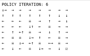
The vanilla policy iteration algorithm solves the Frozen Lake environment in 15 iterations.

Starting from a random policy at iteration 0, we eventually arrive at the optimal policy which is not unique. At iteration 15, going left or down in the first two rows of the map are equally optimal. This is consistent with the known result that the optimal value function is unique, but there can be more than one optimal policy.

What is the effect of the environment on policies?

We can see that applying the exact same DP algorithm on the same map, results in rather different policies if the model of the world is different. In the deterministic case:

In the non-deterministic case:

is_slippery=True: If true the player will move in intended direction with probability of 1/3 else will move in either perpendicular direction with equal probability of 1/3 in both directions.

The policy learnt is one that makes use of the non-deterministic condition; the agent tries very hard to stay away from the lakes and also to move along the map in the far right by facing the border.

Other Notes

How can we be greedy if we have two equally good actions?

If we have two equally good actions and apply a greedy policy with np.argmax, this will always select the first occurrence of highest action. Instead we want to break ties randomly between top scoring actions (still considered greedy).

Do we need to run policy evaluation or policy improvement to convergence each time?

There is some flexibility in the general form of policy iteration (which cycles between evaluation and improvement). Both of these phases can be evaluated partially or fully to convergence, or can involved synchronous or asynchronous updates to the states $v(s), s \in S$. Generalised policy iteration, just involves two interacting processes revolving around approximate policy and approximate value function.

Policy Iteration vs Value Iteration

The greedy approach to finding the policy seems redundant if all it’s doing is taking greedy actions. Value Iteration is a special case of generalised Policy Iteration where we run a single step updating the value function, and then greedify immediately to say that the new $v(s)$ is the value of taking the greedy action. Since there is no reference to a specific policy, we call this simply value iteration. This will still converge to $v*$.

Which “Bellman equation” should I use? Why is “Q-learning” more of a thing than V-learning?

There are two Bellman equations in RL; one for the Q-function (state-action value), and one for the V-function (state value). These are closely related; the Q-function additional incorporates taking an action in a state

\begin{equation} q_{\pi}(s,a)=\sum_{s’, r}p(s’, r \mid s, a)[r + \gamma G_{t+1}(s’)] \end{equation}

whereas the v-function would average across actions in the (stochastic) policy: \begin{equation} v_{\pi}(s) = \sum_a \pi(a \mid s) \sum_{s’, r}p(s’, r \mid s,a)[r + \gamma G_{t+1}(s’)] \end{equation}

Function approximation methods which allow us to estimate $q$ already incorporate the choice of action. As compared to $v$, we do not have to extract the optimal action and explicitly compute the $argmax_a \sum_{s’, r} p(s’ r \mid s, a)$, which requires knowing a model of the environment (transition probability p). This makes conversion to policy more straightforward and therefore Q-learning (function approximation) is known as a model-free RL method.

References

Reinforcement Learning, an Introduction. Chapter 3, 4. Sutton and Barto
Fundamentals of RL; University of Alberta