The Sigmoid in Regression, Neural Network Activation and LSTM Gates
Sigmoid Function in Regression
Logistic Regression is a statistical model which uses a sigmoid (a special case of the logistic) function, $g$ to model the probability of of a binary variable. The function $g$ takes in a linear function with input values $x \in \mathbb{R}^m$ with coefficient weights $b \in \mathbb{R}^m$ and an intercept $b_0$, and ‘squashes’ the output to range from 0 to 1. It is given by
\[\begin{align} X &= b_0 + b_1x_1 + b_2x_2 + \cdots + b_mx_m \\\ g(X) &= \frac{1}{1+e^{-X}} \end{align}\]This function and in logistic regression is used to express the probability $p(y=1|x) = g(X)$, of a binary variable $y$, where $y \in {-1, +1}$.
“Logistic Regression” as a single neuron
This unit appears to be equivalent to a single neuron in a neural network which uses the ‘sigmoid’ activation function applied to $g(w^Tx+b)$, where the bias term $b$ is equivalent to the intercept $b_0$ in logistic regression, and the coefficients $b_1,.. b_m$ is equivalent to the weights $w$ for a single neuron.
From this perspective, if we consider the binary variable to be whether the neuron is activated or not, the output of the neuron is the probability of the neuron being ‘activated’ given inputs. This sounds like a tidy interpretation, but why did the logistic activation fall out of favor as an activation for dnns?
Vanishing Gradient with Sigmoid activation in dnns
The key reason stems from the dynamics of backprop - note that this has nothing to do with the final objective/loss function to optimize but the intermediate activation functions. For logistic regression, we train coefficients by directly following the gradient from the loss, whereas in neural networks we stack multiple layers and train each layer’s weights $w$ and $b$ via chain rule in backdrop.
The implications of stacking multiple layers is that we rely on the gradient flowing through the neural network, and for that there are desirable properties of the outputs of our activation functions, for which the sigmoid activation function is not ideal.
-
“not zero-centered”
-
“computationally less efficient” due to the exp when calculating the derivative
-
Kills gradients when the neuron is “saturated” - when the neuron outputs very high or low values, the gradient is close to 0. Observe in the figure below, the derivative of the sigmoid function, at high and low values, the gradient is close to 0.
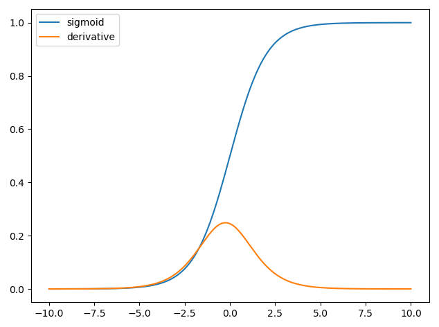
Further, notice that the maximum gradient value we can get from the logistic sigmoid is 0.25, so if the loss were to be backpropagated across multiple layers via the chain rule, the gradient would vanish towards 0 (because we keep multiplying by a number $<1$). For a 100 layer Neural Net, the derivative for weight updates in the first layer $w^{(1)}$ is computed by the following where $a$ are the activations at each layer:
\[\frac{\delta \ell}{\delta w^{(1)}} = \frac{\delta \ell}{\delta a^{(100)}} \frac{\delta a^{(100)}}{\delta a^{(99)}} \cdots \frac{\delta a^{(1)}}{\delta w^{(1)}}\]which would result in a gradient in the order of $0.25^{100}$ - vanishingly small with an increasing number of layers. Since we update weights by $W = W-\alpha \frac{\delta\mathcal{\ell}}{\delta W}$, a gradient of 0 means that we aren’t able to train the network at all.
Handwavy Note: Althought batch normalisation claims to alleviate some of these vanishing gradient problems associated with the Sigmoid function, it seems people still prefer to use other activation functions (such as Relu).
Wait but does LSTM mitigate vanishing and exploding gradients despite still using the sigmoid activation?
Since sigmoid($\sigma$) activation can lead to vanishing gradient problems, why does the LSTM which uses the sigmoid activation ‘mitigate’ vanishing and exploding gradient problems? The key thing to note is how $\sigma$ is used in the updates and the use of $tanh$ for $h_t$.
LSTM equations can be quite intimidating, and they are usually presented with an equally intimidating picture. But let’s focus on the question posed above. The canonical equations are given as:
\[\begin{align} f_t &= \sigma(W_f[h_{t-1}, x_t] + b_f) \\\ i_t &= \sigma(W_i[h_{t-1}, x_t] + b_i) \\\ o_t &= \sigma(W_o [h_{t0}, x_t] + b_o) \end{align}\]In the following, $i$, $f$, and $o$ are used with element wise multiplicative operation $\odot$, that is they have a direct interpretation of being a gate where $0$ corresponds to the gate being closed and $1$ coresponds to the gate being open.
\[\begin{align} g_t &= tanh(W_g[h_t-1, x_t] + b_g) \\\ C_t &= \sigma(f_t \odot C_{t-1} + i_t \odot g_{t}) \\\ h_t &= o_t * tanh(C_t) \end{align}\]$f$, $i$, gates the cells state $c$ with a multiplicative interaction, modulate interaction to the cell state. $o_t$ gates the cell state ‘leaking’ into the hidden state at time step $t$.
Notice that the “hidden state” $h_t$ that gets propagated in future time step, does not use the $\sigma$ activation. Instead, the activation function that modulates the hidden state $h_t$ is $tanh$ and not $\sigma$ . Next, even though for the cell state $C_t$, a sigmoid function is used, the gradient flow is less of an issue, because the cell state $C_t$ gets additively updated (instead of completely replaced).
Nature follows the sigmoid..?
Many natural processes and complex systems exhibit a small rate at the beginning that accelerates and decreases over time.
An example of this is cooperative binding in biochemistry, where binding of an existing ligand is enhanced if there are previous ligands present. The relationship between the ligand concentration and receptor bound is found to be sigmoidal. Hydraulics of river dams, population dynamics etc are also found to be sigmoidal. Learning curves/personal productivity is probably sigmoidal as well. We need some background into the subject before learning accelerates, and then saturates/tapers off.
I suppose that’s why in the absence of an explicit mathematical model, people used the sigmoid function for many years to model a continuous 0 to 1 outcome, before it was discovered that there were problems in the dynamics of backprop. Well, in the early days I suppose learning in artificial neural networks was mostly a heuristic anyway, albeit motivated by statistical mechanics.
References
Kaparthy CS231n Winter 2016: Lecture 5, Lecture 10