Closed form Bayesian Inference for Binomial distributions

Key Concepts

• Bayesian Inference is the use of Bayes theorem to estimate parameters of an unknown probability distribution. The framework uses data to update model beliefs, i.e., the distribution over the parameters of the model.

• A Bernoulli distribution is the discrete probability distribution of a random variable $ X \in \{0, 1\}$ for a single trial. Because there are only two possible outcomes, $P(X=1) = 1-P(X=0)$.

• A Binomial distribution is the probability of observing $k$ “successes”, i.e. no. of times $k=1$ given a sequence of $n$ Bernoulli trials.

• A Beta distribution is the continuous probability distribution of a random variable $\theta \in [0, 1]$. It is the conjugate prior probability distribution for the Bernoulli and Binomial distributions.

Model Preliminaries

In Bayes Theorem, we have some phenomenon that we are trying to represent with a statistical model. The model represents the data-generating process with a probability distribution $p(x|\theta)$, where $\theta$ are the parameters of this model. We start with some prior belief over the values of the parameters, $p(\theta)$, and wish to update out beliefs after observing data $D_n=\{x_1, x_2, .. x_n \}$. By Bayes rule, we can perform the update by:

\begin{equation} p(\theta|D_n) = \frac{p(D_n|\theta)p(\theta)}{p(D_n)} \propto p(D_n|\theta)p(\theta) \end{equation}

• $p(\theta|D_n)$ - posterior probability of $\theta$ after observing $D_n$
• $p(D_n|\theta)$ - likelihood of observing the data under the parameters
• $p(\theta)$ - prior probability of $\theta$ which represents our beliefs
• $p(D_n)$ - marginal likelihood is the probability of seeing the evidence, “marginalised” over all values of $\theta$.

In order to perform an update in eqn(1), we need to have

1. Estimate of the likelihood $p(D_n|\theta)$ and
2. Estimate the prior $p(\theta)$
3. Update the posterior given new observations
   
   

Implementing Bayesian Inference update on the Binomial distribution

1. Estimating the likelihood from a statistical distribution

In a coin toss phenomena, the statistical distribution that represents the data generative process is a binomial distribution.

That is, the likelihood $p(D_n|\theta)$ follows a Binomial distribution with parameters $n$ and $\theta\in[0,1]$, and can be written as $D_n \sim Bin(n, \theta)$. An observation $X$ follows a Bernouli distribution with parameter $\theta$ can be written as $X\sim Ber(\theta)$. For each value that $X$ can take on, $f(x|\theta) = \theta^x(1-\theta)^{1-x}$, for $X\in\{0, 1\}$. Thus, the probability of getting exactly $k$ successes in $n$ trials is given by the probability mass function ${n \choose k} \theta^k (1-\theta)^{n-k}$

import scipy
def calc_likelihood(thetas, n, k):
  pK = scipy.stats.binom(n, thetas).pmf(k)
  #From scipy API, binom.pmf(k) = choose(n, k) * theta^k * (1-theta)^(n-k)
  likelihood = n*pK
  return likelihood

Without the concept of priors, we can get an estimate of $\theta$ by the Maximum Likelihood Estimate (MLE), which is the model parameters that best explains the data observed. $\theta$ that maximises the log-likelihood of the data can be found by setting the derivative to zero.

This is a good idea if we have enough data and the correct model, but if there is insufficient data, MLE can place too much trust in the data observed.

2. Estimating the prior (from a conjugate distribution)

The prior $p(\theta)$ is assumed to come from a beta distribution, with parameters $\alpha$ and $\beta$ can be written as $\theta \sim Beta(\alpha, \beta)$.

A Beta distribution is a family of continuous probability distributions defined on the interval [0, 1]. It’s probability density function is a power function of $\theta$ and $(1-\theta)$, where $nc$ is a normalization constant that ensures total probability integrates to 1.

\(\begin{eqnarray} f(x; \alpha, \beta) = nc.\theta^{\alpha-1}(1-\theta)^{\beta-1} \\ =\frac{\gamma(\alpha+\beta)}{\gamma(\alpha)\gamma(\beta)}\theta^{\alpha-1}(1-\theta)^{\beta-1} \\ \end{eqnarray}\) \begin{equation} =Beta(\alpha, \beta) \end{equation}

def calc_prior(thetas, a, b):
  return scipy.stats.beta(a, b).pdf(thetas)

3. Updating the posterior given new observations

To update the posterior $p(\theta|D_n)$ then becomes

\begin{equation} p(\theta|\alpha, \beta, D_n) \propto p(D_n|\theta).p(\theta|\alpha, \beta) \end{equation}

\begin{equation} \propto \theta^k(1-\theta)^{n-k}.\theta^{\alpha-1}(1-\theta)^{\beta-1} \end{equation}

\begin{equation} = \theta^{k+\alpha-1}(1-\theta)^{n-k+\beta+-1} \end{equation}

With normalization,

\begin{equation} p(\theta|\alpha, \beta, k) = \frac{\gamma(\alpha+n+\beta)}{\gamma(k+\alpha)\gamma(n-k+\beta)}\theta^{k+\alpha-1}(1-\theta)^{n-k+\beta-1}
\end{equation}

\begin{equation} =Beta(\alpha+K, \beta+n-k) \end{equation}

We can perform parameter updates on the posterior by the following $\theta|D_n \sim Beta(\alpha_{new}, \alpha_{old})$, where $\alpha_{new} = (k+\alpha_{old}), \beta_{new} = (n-k+\beta_{old})$

def calc_posterior(thetas, a_old, b_old, n, k):
  a_new = a_old+k
  b_new = b_old+n-k
  posterior = scipy.stats.beta(a_new, b_new).pdf(thetas)
  return posterior, a_new, b_new

We can get multiple estimates from the posterior, including the posterior mean, posterior variance of the parameters, and single parameter estimate from the posterior, the Maximum a Posterior (MAP) estimate: \begin{equation} \theta_{MAP} = argmax_\theta P(\theta|D_n) \end{equation}

Example

1. Without any observations, we start out with the uniform distribution $\theta \sim Beta(\alpha=1, \beta=1)$.
2. Next, we observe 20 data points, 10 of which are successes.

import matplotlib.pyplot as plt
def display_plot(plt):
  plt.xlabel(r'$\theta$', fontsize=14)
  plt.ylabel('Density', fontsize=14)
  plt.legend()
  plt.show()

import numpy as np
a, b = 1, 1
n = 20
k = 10

thetas = np.linspace(0, 1, 500) #generate 500 theta values from 0 to 1 for plotting

prior = calc_prior(thetas, a, b)
posterior, a, b = calc_posterior(thetas, a, b, n, k)
likelihood = calc_likelihood(thetas, n, k)

plt.plot(thetas, prior, label="Prior", c="blue")
plt.plot(thetas, posterior10, label="Posterior_10n", c="red")
plt.plot(thetas, likelihood, label="likelihood", c="green")
display_plot(plt)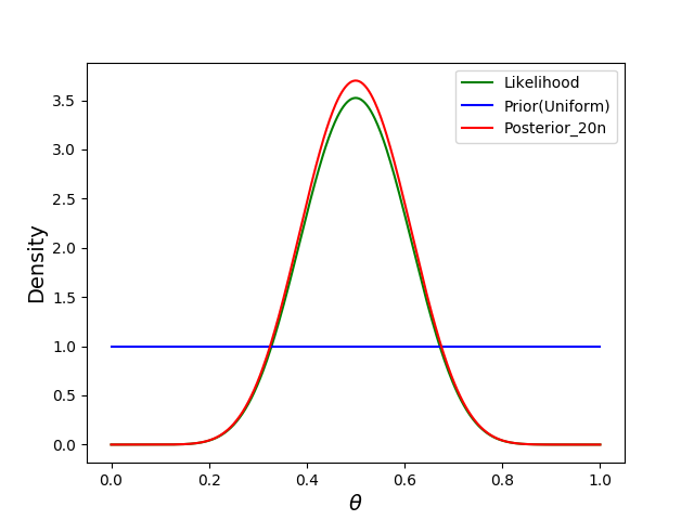

We observe another 100 trials, this time with random likelihood of success

import random
random.seed(0)
n=100
k = np.floor(random.random()*n)

posterior100, a, b = calc_posterior(thetas, a, b, n, k)
likelihood100 = calc_likelihood(thetas, n, k)
plt.plot(thetas, posterior10, label="Prior(Posterior_10n)")
plt.plot(thetas, posterior100, label="Posterior_100n")
plt.plot(thetas, likelihood100, label="Likelihood_100n")
display_plot(plt)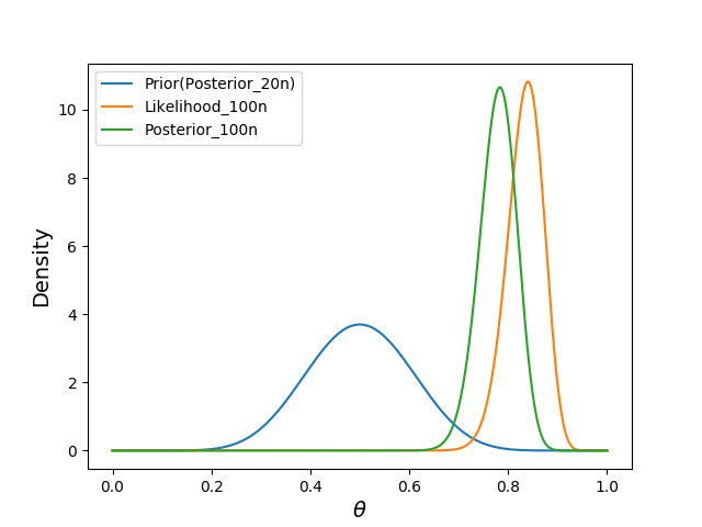

Note that

• our new prior was the previous posterior.
• the likelihood estimate is greater than the posterior, because it does not take into account our prior belief $p(\theta)$.
• In general, the stronger the prior $p(\theta)$, the less the posterior will change subsequently.
• The reason why we had an easy-ish time estimating the posterior, was due to assuming a beta distribution over $\theta$, which is a conjugate prior to the binomial distribution. More on that next time.

References

Beta distribution; Wikipedia
CS598JHM; UIUC/Advanced NLP Spring 10
Computational Statistics; Duke University